Showing posts with label Mathematics_數學. Show all posts

Friday, April 3, 2009

LMA on Python

Python, actually Scipy, provides the Levenberg-Marquardt algortihm for solving least-square problem. It's called leastq in scipy.optimize package. There are a lot's optimization algorithms.
http://docs.scipy.org/doc/scipy/reference/optimize.html

Basically, It was coded by fortran. http://www.netlib.org/minpack/
You can download the test code for fortran version form http://www1.fpl.fs.fed.us/minpack.ls.test.html

You can use it directly by calling "scipy.optimize.leastsq" after including "from scipy.optimize import leastsq"

These are good simple examples.


Reminder:
Be careful the arrary usage of input data x and y.

Wednesday, March 4, 2009

The method of solving least-squares problems

Linear least squares problems
  • Newton's Method
Non-Linear least squares problems
  • Gauss-Newton Method
  • Quasi-Newton Method
  • Gauss-Raphson Method
  • Levenberg-Marguardt Method
  • Powell's Dog Leg Method
  • Hybrid Method: L-M and Quasi-Newton
Good references:
  • 1999, Poul E. Frandsen, http://www2.imm.dtu.dk/documents/ftp/publlec/lec2_99.pdf
Descent method
Conjugate Gradient mehod
Newton-based method, included Quasi-Newton
  • 1999, Hans B. Nielsen: http://www2.imm.dtu.dk/documents/ftp/tr99/tr05_99.pdf
Descent method
Gauss-Newton method
Levenberg-Marquardt method
Powell's Dog Leg method
Hybrid: LMA+QN
Newton's Method, NM
Also called Newton-Raphson Method.  It uses the first few terms of the Taylor series (Taylor expansion) of a function  in the vicinity of a suspected root.  
  • http://mathworld.wolfram.com/NewtonsMethod.html
  • http://en.wikipedia.org/wiki/Newton's_method

Relationship between Newton's method, Halley method, and Householder's method.
  • Newton's method is 1st in the class of Householder's method.
  • Halley's method is 2nd in the class of Householder's method.
  • http://en.wikipedia.org/wiki/Householder's_method
  • http://en.wikipedia.org/wiki/Halley's_method

  • Levenberg-Marquardt Algorithm, LMA
  • http://en.wikipedia.org/wiki/Levenberg-Marquardt_algorithm
  • http://mathworld.wolfram.com/Levenberg-MarquardtMethod.html
  • http://homepages.inf.ed.ac.uk/cgi/rbf/CVONLINE/entries.pl?TAG49
  • Nov. 1996, Sam Roweis: http://www.cs.toronto.edu/~roweis/notes/lm.pdf
  • Good Introduction to talk about the LM from Newton's method, modefied by Levenberg, then modefied by Marquardt to become LM algorithm.
1999, Hans B. Nielsen: http://www2.imm.dtu.dk/documents/ftp/tr99/tr05_99.pdf
Apr. 2004, Hans B. Nielsen: http://www.imm.dtu.dk/pubdb/views/edoc_download.php/3215/pdf/imm3215.pdf
  • Above two articles are refered by LEVMAR.
June 2004, Ananth R.: http://www.cc.gatech.edu/~ananth/docs/lmtut.pdf
  • A good article also to talk about the LM from Newton's, Levenberg, and Marquardt to become LMA.
Feb. 2005, Manolis L.: http://www.ics.forth.gr/~lourakis/levmar/levmar.pdf
  • The article talking about source code LEVMAR. A pseudocode provided.
Nov. 2006, Pradit M.: http://cobweb.ecn.purdue.edu/~kak/courses-i-teach/ECE661.08/homework/HW5_LM_handout.pdf
  • Simple example and Matlab code provided.
http://www.cse.ucsd.edu/classes/fa04/cse252c/vrabaud1.pdf
  • Matlab code, thanks for Pradit Mittrapiyanuruk.

Gauss-Newton Method, GNM
  • http://en.wikipedia.org/wiki/Gauss-Newton_algorithm
  • http://reference.wolfram.com/mathematica/tutorial/UnconstrainedOptimizationGaussNewtonMethods.html
  • 1999, Hans B. Nielsen: http://www2.imm.dtu.dk/documents/ftp/tr99/tr05_99.pdf
Gauss-Raphson Method, GRM
Continue..
Quasi-Netwon Method, QNM
  • http://reference.wolfram.com/mathematica/tutorial/UnconstrainedOptimizationQuasiNewtonMethods.html
  • 1999, Poul E. Frandsen, http://www2.imm.dtu.dk/documents/ftp/publlec/lec2_99.pdf
Powell's Dog Leg Method, PDLM
  • 1999, Hans B. Nielsen: http://www2.imm.dtu.dk/documents/ftp/tr99/tr05_99.pdf
Hybrid Method: L-M and Quasi-Newton, H:LM+QN
  • 1999, Hans B. Nielsen: http://www2.imm.dtu.dk/documents/ftp/tr99/tr05_99.pdf
LMA for linear convergence
QN for superlinear convergence
Papers:
  • Yao Jianchao, Chia Tien Chern, COMPARISON OF NEWTON-GAUSS WITH LEVENBERG-MARQUARDT ALGORITHM FOR SPACE RESECTION, Proc. ACRS 2001 - 22nd Asian Conference on Remote Sensing, 5-9 November 2001, Singapore. Vol. 1, pp. 256-261.
  • C. Kanzow, N. Yamashita and M. Fukushima, Levenberg–Marquardt methods with strong local convergence properties for solving nonlinear equations with convex constraints, J. Comput. Appl. Math.172 (2004), pp. 375–397.
  • Kanzow, C., Yamashita, N., and Fukushima, M. 2004. Levenberg-Marquardt methods with strong local convergence properties for solving nonlinear equations with convex constraints. J. Comput. Appl. Math. 172, 2 (Dec. 2004), 375-397. DOI= http://dx.doi.org/10.1016/j.cam.2004.02.013
  • Lourakis, M. I. and Argyros, A. A. 2005. Is Levenberg-Marquardt the Most Efficient Optimization Algorithm for Implementing Bundle Adjustment?. In Proceedings of the Tenth IEEE international Conference on Computer Vision - Volume 2 (October 17 - 20, 2005). ICCV. IEEE Computer Society, Washington, DC, 1526-1531. DOI= http://dx.doi.org/10.1109/ICCV.2005.128

Source codes:
levmar: Levenberg-Marquardt nonlinear least squares algorithms in C/C++
lmfit — a C/C++ routine for Levenberg-Marquardt minimization with wrapper for least-squares curve fitting
lmfit is easy to install it because it is without the dependency problem.
Levenberg-Marquardt for Visual C++ 2005
Levenberg-Marquardt algorithm for multivariate optimization in C#/C++/Delphi/VB6/Zonnon

Continue....

Tuesday, March 3, 2009

Simple Matlab demo of LM algorithm

Special thanks to Pradit Mittrapiyanuruk.
His open article gives us a very good simple demo of Levenberg-Marquardt Algorithm.

The code is almost the same with code provided from http://www.cse.ucsd.edu/classes/fa04/cse252c/vrabaud1.pdf
The red statements are simple plotting graphic. The statements will show the result as iteration=1,2,3,5,10, and 100.
=================================================================
%definition, giving a function f and create jacobian function for function
%f
syms a b x y real;
f=( a * cos(b*x) + b * sin(a*x))
d=y-f;
Jsym=jacobian(d,[a b]);
%Generate the synthetic data from the curve function with some additional
%noise
a=100;
b=102;
x=[0:0.1:2*pi]';
y = a * cos(b*x) + b * sin(a*x);
% add random noise
y_input = y + 5*rand(length(x),1);

%start the LMA
% initial guess for the parameters
a0=100.5; b0=102.5;
y_init = a0 * cos(b0*x) + b0 * sin(a0*x);
Ndata=length(y_input);
Nparams=2; % a and b are the parameters to be estimated
n_iters=100; % set # of iterations for the LM
lamda=0.01; % set an initial value of the damping factor for the LM
updateJ=1;
a_est=a0;
b_est=b0;
for it=1:n_iters
if updateJ==1
% Evaluate the Jacobian matrix at the current parameters (a_est, b_est)
J=zeros(Ndata,Nparams);
for i=1:length(x)
J(i,:)=[-cos(b_est*x(i))-(b_est*cos(a_est*x(i))*x(i)) (a_est*sin(b_est*x(i))*x(i))-sin(a_est*x(i))];
end
% Evaluate the distance error at the current parameters
y_est = a_est * cos(b_est*x) + b_est * sin(a_est*x);
d=y_input-y_est;
% compute the approximated Hessian matrix, J’ is the transpose of J
H=J'*J;
if it==1 % the first iteration : compute the total error
e=dot(d,d);
end
end

% Apply the damping factor to the Hessian matrix
H_lm=H+(lamda*eye(Nparams,Nparams));
% Compute the updated parameters
dp=-inv(H_lm)*(J'*d(:));
a_lm=a_est+dp(1);
b_lm=b_est+dp(2);
% Evaluate the total distance error at the updated parameters
y_est_lm = a_lm * cos(b_lm*x) + b_lm * sin(a_lm*x);
% plot
if it == 1
h1=plot(y_input, 'b');
hold on
h1=plot(y_est_lm, 'r');
legend(h1,'iteration=1');
hold off
pause
end
if it == 2
h1=plot(y_input, 'b');
hold on
h1=plot(y_est_lm, 'r');
legend(h1,'iteration=2');
hold off
pause
end
if it == 3
h1=plot(y_input, 'b');
hold on
h1=plot(y_est_lm, 'r');
legend(h1,'iteration=3');
hold off
pause
end
if it == 5
h1=plot(y_input, 'b');
hold on
h1=plot(y_est_lm, 'r');
legend(h1,'iteration=5');
hold off
pause
end
if it == 10
h2=plot(y_input, 'b');
hold on
h2=plot(y_est_lm, 'r');
legend(h2,'iteration=10');
hold off
pause
end
if it == 100
h3=plot(y_input, 'b');
hold on
h3=plot(y_est_lm, 'r');
legend(h3,'iteration=100');
hold off
pause
end
d_lm=y_input-y_est_lm;
e_lm=dot(d_lm,d_lm);
% If the total distance error of the updated parameters is less than the previous one
% then makes the updated parameters to be the current parameters
% and decreases the value of the damping factor
if e_lm
lamda=lamda/10;
a_est=a_lm;
b_est=b_lm;
e=e_lm;
disp(e);
updateJ=1;
else % otherwise increases the value of the damping factor
updateJ=0;
lamda=lamda*10;
end
end
=================================================================
Code download, lmademo.m
You will the blue line is fitting close to red line after few iterations.


Monday, December 22, 2008

Gradient, Hessian, and Jacobian

The problem
A set y=f(x) of m equations in n variable x1,...,xn
f  
The first-order partial derivatives of a vector-valued function, so called Jacobian, or Jacobian Matrix, matrix size is n x m.

The problem 
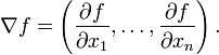
A set y=f(x) of 1 equations in n variable x1,...,xn
f  
The first-order partial derivatives of a vector-valued function, so called Gradient, or Gradient vector. Matrix size is 1 x n.


The second-order partial derivatives of a vector-valued function, so called Hessain, or Hessain Matrix. Matrix size is n x n.

Monday, December 15, 2008

Taylor Series

Taylor Series = Taylor Expansion = Taylor Series Expansion.

Brief introduction video in Chinese


Perfect Demo
Other Demo

Wednesday, March 5, 2008

算術平均數(mean),幾何平均數(Geometric mean),調和平均數(Harmoic mean)

兩數X1,X2的算術平均數(mean, arithmetic average) = (X1+X2)/2
兩數X1,X2的幾何平均數(Geometric mean) = sqaure(X1*X2)
兩數X1,X2的調和平均數(Harmonic mean) = 2*X1*x2/(X1+X2)
兩數X1,X2的平方平均數(Quadratic mean) = square((X1^2+X2^2)/2)

Thursday, November 15, 2007

Clicky

Clicky Web Analytics