Simple Matlab demo of LM algorithm

Special thanks to Pradit Mittrapiyanuruk.

His open article gives us a very good simple demo of Levenberg-Marquardt Algorithm.

The code is almost the same with code provided from http://www.cse.ucsd.edu/classes/fa04/cse252c/vrabaud1.pdf

The red statements are simple plotting graphic. The statements will show the result as iteration=1,2,3,5,10, and 100.

=================================================================

%definition, giving a function f and create jacobian function for function

%f

syms a b x y real;

f=( a * cos(b*x) + b * sin(a*x))

d=y-f;

Jsym=jacobian(d,[a b]);

%Generate the synthetic data from the curve function with some additional

%noise

a=100;

b=102;

x=[0:0.1:2*pi]';

y = a * cos(b*x) + b * sin(a*x);

% add random noise

y_input = y + 5*rand(length(x),1);

%start the LMA

% initial guess for the parameters

a0=100.5; b0=102.5;

y_init = a0 * cos(b0*x) + b0 * sin(a0*x);

Ndata=length(y_input);

Nparams=2; % a and b are the parameters to be estimated

n_iters=100; % set # of iterations for the LM

lamda=0.01; % set an initial value of the damping factor for the LM

updateJ=1;

a_est=a0;

b_est=b0;

for it=1:n_iters

if updateJ==1

% Evaluate the Jacobian matrix at the current parameters (a_est, b_est)

J=zeros(Ndata,Nparams);

for i=1:length(x)

J(i,:)=[-cos(b_est*x(i))-(b_est*cos(a_est*x(i))*x(i)) (a_est*sin(b_est*x(i))*x(i))-sin(a_est*x(i))];

end

% Evaluate the distance error at the current parameters

y_est = a_est * cos(b_est*x) + b_est * sin(a_est*x);

d=y_input-y_est;

% compute the approximated Hessian matrix, J’ is the transpose of J

H=J'*J;

if it==1 % the first iteration : compute the total error

e=dot(d,d);

end

end

% Apply the damping factor to the Hessian matrix

H_lm=H+(lamda*eye(Nparams,Nparams));

% Compute the updated parameters

dp=-inv(H_lm)*(J'*d(:));

a_lm=a_est+dp(1);

b_lm=b_est+dp(2);

% Evaluate the total distance error at the updated parameters

y_est_lm = a_lm * cos(b_lm*x) + b_lm * sin(a_lm*x);

% plot

if it == 1

h1=plot(y_input, 'b');

hold on

h1=plot(y_est_lm, 'r');

legend(h1,'iteration=1');

hold off

pause

end

if it == 2

h1=plot(y_input, 'b');

hold on

h1=plot(y_est_lm, 'r');

legend(h1,'iteration=2');

hold off

pause

end

if it == 3

h1=plot(y_input, 'b');

hold on

h1=plot(y_est_lm, 'r');

legend(h1,'iteration=3');

hold off

pause

end

if it == 5

h1=plot(y_input, 'b');

hold on

h1=plot(y_est_lm, 'r');

legend(h1,'iteration=5');

hold off

pause

end

if it == 10

h2=plot(y_input, 'b');

hold on

h2=plot(y_est_lm, 'r');

legend(h2,'iteration=10');

hold off

pause

end

if it == 100

h3=plot(y_input, 'b');

hold on

h3=plot(y_est_lm, 'r');

legend(h3,'iteration=100');

hold off

pause

end

d_lm=y_input-y_est_lm;

e_lm=dot(d_lm,d_lm);

% If the total distance error of the updated parameters is less than the previous one

% then makes the updated parameters to be the current parameters

% and decreases the value of the damping factor

if e_lm

lamda=lamda/10;

a_est=a_lm;

b_est=b_lm;

e=e_lm;

disp(e);

updateJ=1;

else % otherwise increases the value of the damping factor

updateJ=0;

lamda=lamda*10;

end

end

=================================================================

Code download, lmademo.m

You will the blue line is fitting close to red line after few iterations.

HTK Chapter 3 - Section 2 - Step 7

Below paragraphs are belong to

• HTKBooks, 
  
• 苏统华, 哈尔滨工业大学人工智能研究室, 2006年10月30日, 
  
• Howard Hung-Ju Chou, Intelligence Information Retrieval Lab., NCKU, Taiwan(R.O.C.).
  

Environment:

• HTK 3.4 
  
• Cygwin NT-5.1 1.5.25
  

Section 2 is Creating Monophone HMMs - 建立單音素模型

• Step 6 - Creating Flat Start Monophones
  
• Step 7 - Fixing the Slience Models
  
• Step 8 - Realigning the Training Data

In Step 6, we generate hmm0, hmm1, hmm2, with slience model "sil".

Now the tutorial teaching us to model the model in Fig. 3.9 in Subsection 3.2.2 in HTK Books.

Physical meaning,....

Create a 3 state model for "sp", so we just only one non-emtting state for "sp" model.

How to do that?

1. Use text editor to...
2. Use HHEd

The content of "sil" is 

=================================================================

~h "sil"

<  BEGINHMM  >

<  NUMSTATES  > 5

<  STATE  > 2

<> 39

 -9.389361e-001 -1.287944e+000 8.473723e-002 -4.411200e+000 5.332393e-001 1.843251e-001 2.939802e+000 -2.362492e+000 3.039350e-001 5.898609e-003 -3.105349e+000 -1.462931e+000 5.539479e+001 -2.752953e-002 -2.782337e-002 5.648132e-003 4.534409e-002 1.876847e-002 2.492056e-002 1.361921e-002 -1.723138e-002 1.886967e-002 3.497830e-002 1.276191e-002 2.784961e-002 -3.208526e-002 3.180009e-004 1.971325e-003 -3.830043e-003 -1.048350e-002 -1.810746e-003 -1.773861e-003 -9.375007e-004 3.254613e-004 8.180511e-004 3.765909e-003 1.624564e-003 -3.620259e-004 3.278390e-003

<  VARIANCE  > 39

 4.180664e+001 3.271134e+001 3.581472e+001 6.693031e+001 3.528064e+001 5.052157e+001 2.934049e+001 3.423428e+001 3.710680e+001 3.691701e+001 3.710829e+001 2.969890e+001 6.507053e+001 1.337987e+000 1.072017e+000 1.307518e+000 1.887581e+000 1.697909e+000 1.890241e+000 1.785829e+000 2.181937e+000 1.875866e+000 1.797650e+000 1.730149e+000 1.642454e+000 9.926388e-001 1.710149e-001 1.462792e-001 1.848170e-001 2.626473e-001 2.605441e-001 2.970572e-001 3.222261e-001 3.782587e-001 3.125882e-001 3.063583e-001 2.895371e-001 2.911398e-001 1.187189e-001

<  GCONST  > 1.071964e+002

<  STATE  > 3

<  MEAN  > 39

 -1.991913e+000 -4.775551e-002 2.959489e+000 2.209434e+000 2.078557e+000 5.562240e+000 5.464221e+000 -4.776323e+000 1.673594e+000 2.683963e+000 -4.633354e+000 -9.166243e-001 4.628856e+001 -1.207492e-001 -8.760695e-002 -7.070365e-002 7.516075e-002 -4.011013e-003 3.128541e-002 8.115381e-002 -3.286631e-002 1.295639e-001 1.558424e-001 5.380721e-002 1.054287e-001 -1.449030e-001 1.667164e-002 2.022874e-002 1.105829e-003 -2.183086e-002 -7.496935e-003 -4.172942e-002 -3.657551e-002 1.193289e-002 -1.476659e-002 -2.710904e-002 1.349834e-002 9.330045e-004 2.211097e-002

<  VARIANCE  > 39

 5.752877e+000 5.706749e+000 9.791572e+000 1.276698e+001 1.414043e+001 1.682921e+001 1.643664e+001 1.884838e+001 1.942560e+001 2.041147e+001 1.927709e+001 1.510888e+001 1.051241e+001 2.168639e-001 3.732721e-001 6.485465e-001 8.246439e-001 9.308486e-001 1.138545e+000 1.447520e+000 1.688959e+000 1.681041e+000 1.680561e+000 1.580671e+000 1.330634e+000 9.859556e-002 3.477598e-002 6.478215e-002 1.191088e-001 1.600942e-001 1.801341e-001 2.153407e-001 2.852951e-001 3.301157e-001 3.403606e-001 3.369383e-001 3.197604e-001 2.676942e-001 1.323066e-002

7.787578e+001

<  STATE  > 4

<  MEAN  > 39

 -2.982345e+000 -1.252340e+000 1.087486e+000 7.909203e-001 1.536108e+000 3.573169e+000 5.625374e+000 -3.234990e+000 2.314626e+000 3.188504e+000 -9.258319e-001 1.509047e+000 4.699720e+001 -7.613304e-003 5.702919e-003 -6.563795e-003 -4.346590e-003 -7.446251e-003 -8.997340e-003 -3.822424e-003 -2.726374e-003 -3.682886e-003 -1.174716e-003 1.001520e-002 1.304566e-002 -2.283418e-003 -2.802775e-004 1.980037e-003 1.587337e-003 -6.755204e-004 2.919145e-003 1.646213e-003 -1.079046e-004 1.305768e-003 2.884402e-004 -2.650670e-003 -2.699222e-003 -4.054980e-003 3.949025e-003

<  VARIANCE  > 39

 5.313723e+000 4.299637e+000 5.806711e+000 7.572632e+000 1.195562e+001 1.127259e+001 1.345822e+001 1.842092e+001 1.902783e+001 1.841946e+001 1.679353e+001 1.275744e+001 2.541775e+000 1.125962e-001 2.241242e-001 3.554686e-001 4.804470e-001 7.102868e-001 8.679712e-001 1.053879e+000 1.259253e+000 1.247817e+000 1.199414e+000 1.138910e+000 9.791774e-001 7.236452e-002 2.274701e-002 4.417740e-002 7.068438e-002 9.644291e-002 1.455498e-001 1.809241e-001 2.171511e-001 2.593471e-001 2.625059e-001 2.464305e-001 2.333392e-001 2.013770e-001 1.429966e-002

<  GCONST  > 6.495581e+001

<  TRANSP  > 5

 0.000000e+000 1.000000e+000 0.000000e+000 0.000000e+000 0.000000e+000

 0.000000e+000 9.399074e-001 6.009261e-002 0.000000e+000 0.000000e+000

 0.000000e+000 0.000000e+000 8.703428e-001 1.296572e-001 0.000000e+000

 0.000000e+000 0.000000e+000 0.000000e+000 9.800954e-001 1.990458e-002

 0.000000e+000 0.000000e+000 0.000000e+000 0.000000e+000 0.000000e+000

<  ENDHMM  >

=================================================================

We copy the red statements to be model of "sp", but remember that only 3 state exist in model "sp" so we have to modify to 2.

=======================================================================

~h "sp"

<  BEGINHMM  >

<  NUMSTATES  > 3

<  STATE  > 2

<  MEAN  > 39

 -9.389361e-001 -1.287944e+000 8.473723e-002 -4.411200e+000 5.332393e-001 1.843251e-001 2.939802e+000 -2.362492e+000 3.039350e-001 5.898609e-003 -3.105349e+000 -1.462931e+000 5.539479e+001 -2.752953e-002 -2.782337e-002 5.648132e-003 4.534409e-002 1.876847e-002 2.492056e-002 1.361921e-002 -1.723138e-002 1.886967e-002 3.497830e-002 1.276191e-002 2.784961e-002 -3.208526e-002 3.180009e-004 1.971325e-003 -3.830043e-003 -1.048350e-002 -1.810746e-003 -1.773861e-003 -9.375007e-004 3.254613e-004 8.180511e-004 3.765909e-003 1.624564e-003 -3.620259e-004 3.278390e-003

<  VARIANCE  > 39

 4.180664e+001 3.271134e+001 3.581472e+001 6.693031e+001 3.528064e+001 5.052157e+001 2.934049e+001 3.423428e+001 3.710680e+001 3.691701e+001 3.710829e+001 2.969890e+001 6.507053e+001 1.337987e+000 1.072017e+000 1.307518e+000 1.887581e+000 1.697909e+000 1.890241e+000 1.785829e+000 2.181937e+000 1.875866e+000 1.797650e+000 1.730149e+000 1.642454e+000 9.926388e-001 1.710149e-001 1.462792e-001 1.848170e-001 2.626473e-001 2.605441e-001 2.970572e-001 3.222261e-001 3.782587e-001 3.125882e-001 3.063583e-001 2.895371e-001 2.911398e-001 1.187189e-001

<  GCONST  > 1.071964e+002

<  TRANSP  > 3

 0.000000e+000 1.000000e+000 0.000000e+000

 0.000000e+000 8.703428e-001 1.296572e-001

 0.000000e+000 0.000000e+000 0.000000e+000

<  ENDHMM  >

=======================================================================

Then use HHEd to modefy hmm4/macros and hmm4/hmmdefs accroding the edit commands in sil.hed.

--------------------------------------------------------------------------------------------------------------------

$ HHEd -H ./hmms/hmm4/macros -H ./hmms/hmm4/hmmdefs -M ./hmms/hmm5 sil.hed ./lists/monophones1

--------------------------------------------------------------------------------------------------------------------

The new hmmdefs, will be added the following statements,

======================================================================================

~s "silst"

<  MEAN  > 39

 -9.389361e-01 -1.287944e+00 8.473723e-02 -4.411200e+00 5.332393e-01 1.843251e-01 2.939802e+00 -2.362492e+00 3.039350e-01 5.898609e-03 -3.105349e+00 -1.462931e+00 5.539479e+01 -2.752953e-02 -2.782337e-02 5.648132e-03 4.534409e-02 1.876847e-02 2.492056e-02 1.361921e-02 -1.723138e-02 1.886967e-02 3.497830e-02 1.276191e-02 2.784961e-02 -3.208526e-02 3.180009e-04 1.971325e-03 -3.830043e-03 -1.048350e-02 -1.810746e-03 -1.773861e-03 -9.375007e-04 3.254613e-04 8.180511e-04 3.765909e-03 1.624564e-03 -3.620259e-04 3.278390e-03

39

 4.180664e+01 3.271134e+01 3.581472e+01 6.693031e+01 3.528064e+01 5.052157e+01 2.934049e+01 3.423428e+01 3.710680e+01 3.691701e+01 3.710829e+01 2.969890e+01 6.507053e+01 1.337987e+00 1.072017e+00 1.307518e+00 1.887581e+00 1.697909e+00 1.890241e+00 1.785829e+00 2.181937e+00 1.875866e+00 1.797650e+00 1.730149e+00 1.642454e+00 9.926388e-01 1.710149e-01 1.462792e-01 1.848170e-01 2.626473e-01 2.605441e-01 2.970572e-01 3.222261e-01 3.782587e-01 3.125882e-01 3.063583e-01 2.895371e-01 2.911398e-01 1.187189e-01

<  GCONST  > 1.071964e+02

======================================================================================

And original ~h "sil" and ~h "sp" become to be like following,

====================================================

~h "sp"

3

2

~s "silst"

3

 0.000000e+00 7.000000e-01 3.000000e-01

 0.000000e+00 8.703428e-01 1.296572e-01

 0.000000e+00 0.000000e+00 0.000000e+00

~h "sil"

<  BEGINHMM  >

<  NUMSTATES  > 5

<  STATE  > 2

<  MEAN  > 39

 -9.389361e-01 -1.287944e+00 8.473723e-02 -4.411200e+00 5.332393e-01 1.843251e-01 2.939802e+00 -2.362492e+00 3.039350e-01 5.898609e-03 -3.105349e+00 -1.462931e+00 5.539479e+01 -2.752953e-02 -2.782337e-02 5.648132e-03 4.534409e-02 1.876847e-02 2.492056e-02 1.361921e-02 -1.723138e-02 1.886967e-02 3.497830e-02 1.276191e-02 2.784961e-02 -3.208526e-02 3.180009e-04 1.971325e-03 -3.830043e-03 -1.048350e-02 -1.810746e-03 -1.773861e-03 -9.375007e-04 3.254613e-04 8.180511e-04 3.765909e-03 1.624564e-03 -3.620259e-04 3.278390e-03

<  VARIANCE  > 39

 4.180664e+01 3.271134e+01 3.581472e+01 6.693031e+01 3.528064e+01 5.052157e+01 2.934049e+01 3.423428e+01 3.710680e+01 3.691701e+01 3.710829e+01 2.969890e+01 6.507053e+01 1.337987e+00 1.072017e+00 1.307518e+00 1.887581e+00 1.697909e+00 1.890241e+00 1.785829e+00 2.181937e+00 1.875866e+00 1.797650e+00 1.730149e+00 1.642454e+00 9.926388e-01 1.710149e-01 1.462792e-01 1.848170e-01 2.626473e-01 2.605441e-01 2.970572e-01 3.222261e-01 3.782587e-01 3.125882e-01 3.063583e-01 2.895371e-01 2.911398e-01 1.187189e-01

<  GCONST  > 1.071964e+02

3

~s "silst"

<  STATE  > 4

<  MEAN  > 39

 -2.982345e+00 -1.252340e+00 1.087486e+00 7.909203e-01 1.536108e+00 3.573169e+00 5.625374e+00 -3.234990e+00 2.314626e+00 3.188504e+00 -9.258319e-01 1.509047e+00 4.699720e+01 -7.613304e-03 5.702919e-03 -6.563795e-03 -4.346590e-03 -7.446251e-03 -8.997340e-03 -3.822424e-03 -2.726374e-03 -3.682886e-03 -1.174716e-03 1.001520e-02 1.304566e-02 -2.283418e-03 -2.802775e-04 1.980037e-03 1.587337e-03 -6.755204e-04 2.919145e-03 1.646213e-03 -1.079046e-04 1.305768e-03 2.884402e-04 -2.650670e-03 -2.699222e-03 -4.054980e-03 3.949025e-03

<  VARIANCE  > 39

 5.313723e+00 4.299637e+00 5.806711e+00 7.572632e+00 1.195562e+01 1.127259e+01 1.345822e+01 1.842092e+01 1.902783e+01 1.841946e+01 1.679353e+01 1.275744e+01 2.541775e+00 1.125962e-01 2.241242e-01 3.554686e-01 4.804470e-01 7.102868e-01 8.679712e-01 1.053879e+00 1.259253e+00 1.247817e+00 1.199414e+00 1.138910e+00 9.791774e-01 7.236452e-02 2.274701e-02 4.417740e-02 7.068438e-02 9.644291e-02 1.455498e-01 1.809241e-01 2.171511e-01 2.593471e-01 2.625059e-01 2.464305e-01 2.333392e-01 2.013770e-01 1.429966e-02

<  GCONST  > 6.495583e+01

<  TRANSP  > 5

 0.000000e+00 1.000000e+00 0.000000e+00 0.000000e+00 0.000000e+00

 0.000000e+00 7.519259e-01 4.807409e-02 2.000000e-01 0.000000e+00

 0.000000e+00 0.000000e+00 8.703428e-01 1.296572e-01 0.000000e+00

 0.000000e+00 2.000000e-01 0.000000e+00 7.840764e-01 1.592367e-02

 0.000000e+00 0.000000e+00 0.000000e+00 0.000000e+00 0.000000e+00

<  ENDHMM  >

==================================================== 

Because the commands in sil.hed,

============================

AT  2  4  0.2 { sil. transp }

AT  4  2  0.2 { sil. transp }

AT  1  3  0.3 { sp. transp }

TI slist { sil.state[3], sp.state[2] }

============================

AT  i  j  prob  itemList(t) in page 256 in HTKBook 3.4.

The probability will be rescaled so that summation of p is equal to 1.0.

For example in ~h "sp",

We modify it by AT   1  3  0.3 { sp.transp }, so the sp.transp 

==================================

<  TRANSP  > 3

 0.000000e+000 1.000000e+000 0.000000e+000

 0.000000e+000 8.703428e-001 1.296572e-001

 0.000000e+000 0.000000e+000 0.000000e+000

==================================

to be rescaled to 

==================================

<  TRANSP  > 3

 0.000000e+00 7.000000e-01 3.000000e-01

 0.000000e+00 8.703428e-01 1.296572e-01

 0.000000e+00 0.000000e+00 0.000000e+00

==================================

TI means Tie itemlist to be macroname.

-------------------------------------

$ Ti  macroname  itemlist

-------------------------------------

To know more about TI command, please refer to Chapter 10.3 in HTK Book. (PS: the section 10.3 and section 10.4 should be exchanged.)

To know more about HHed, please refer to Chapter 10 in HTK Book.

Continue...

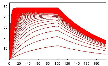
Memo to use CLAMP to generate simulation data

Feel free to use the model save file, named "generate_100_200_0.25.mdl"

Aother one is the same with the tutorial, named "generate_6_200_0.25.mdl"

Download from HERE.

"generate_100_200_0.25.mdl" means

• Number of curves: 100 
• Total time: 200 seconds
• Sample interval: 0.25
• Concentration is 1, 0.99, 0.98~0.01
• Injection time: 100 seconds

Generate simulation file with noise fast,

1. Selection add noise, choose the value you want
2. Save the file to be "Save sim"
3. Click model page
4. Press Simulation again
5. You will recover the data with no noise

標點符號的英文

相信一定有人跟我一樣，英文不是很好。

看到一些文件，會看到各式各樣的符號，然後也不太熟悉，所以這些網頁到是整理不少符號。

http://www.eol.cn/article/20060227/3175182.shtml

http://www.hoyo.idv.tw/78/english-comma.htm

http://pub.thit.edu.tw/ThitCC/邱世芬老師/doc/3-1-6/3-1-6-2.htm

http://www.grammarbook.com/

HTK Chapter 3 - Section 2 - Step 6

Below paragraphs are belong to

• HTKBooks, 
  
• 苏统华, 哈尔滨工业大学人工智能研究室, 2006年10月30日, 
  
• Howard Hung-Ju Chou, Intelligence Information Retrieval Lab., NCKU, Taiwan(R.O.C.).
  

Environment:

• HTK 3.4 
  
• Cygwin NT-5.1 1.5.25
  

Section 2 is Creating Monophone HMMs - 建立單音素模型

• Step 6 - Creating Flat Start Monophones
  
• Step 7 - Fixing the Slience Models
  
• Step 8 - Realigning the Training Data
  

Now, we have the feature vectors of training data and testing data.
.\data\train\feature\S0001.mfcc
.\data\train\feature\S0002.mfcc
.\data\train\feature\S0003.mfcc
.\data\train\feature\S0004.mfcc
.\data\train\feature\S0005.mfcc
.\data\train\feature\S0006.mfcc
.\data\train\feature\S0007.mfcc
.\data\train\feature\S0008.mfcc
.\data\train\feature\S0009.mfcc
....so no. It is Training data.

Testing data is following,
.\data\test\feature\T0001.mfc
.\data\test\feature\T0002.mfc
.\data\test\feature\T0003.mfc
.\data\test\feature\T0004.mfc
.\data\test\feature\T0005.mfc
.\data\test\feature\T0006.mfc
.\data\test\feature\T0007.mfc
.\data\test\feature\T0008.mfc
.\data\test\feature\T0009.mfc

Next step, we have to give HTK a known prototype HMM model, and give initial value for parameters of model which we use.
=============================

~o <  VecSize  > 39 <  MFCC_0_D_A  >

~h "proto"

<  BeginHMM  >

  <  NumStates  > 5

  <  State  > 2

    <  Mean  > 39

      0.0 0.0 0.0 0.0 0.0 0.0 0.0 0.0 0.0 0.0 0.0 0.0 0.0 0.0 0.0 0.0 0.0 0.0 0.0 0.0 0.0 0.0 0.0 0.0 0.0 0.0 0.0 0.0 0.0 0.0 0.0 0.0 0.0 0.0 0.0 0.0 0.0 0.0 0.0 

    <  Variance  > 39

      1.0 1.0 1.0 1.0 1.0 1.0 1.0 1.0 1.0 1.0 1.0 1.0 1.0 1.0 1.0 1.0 1.0 1.0 1.0 1.0 1.0 1.0 1.0 1.0 1.0 1.0 1.0 1.0 1.0 1.0 1.0 1.0 1.0 1.0 1.0 1.0 1.0 1.0 1.0

 <  State  > 3

    <  Mean  > 39

      0.0  (x39) it's like state 2 

    <  Variance  > 39

      1.0 (x39)

 <  State  > 4

    <  Mean  > 39

      0.0  (x39) 

    <  Variance  > 39

      1.0  (x39)

 <  TransP  > 5

  0.0 1.0 0.0 0.0 0.0

  0.0 0.6 0.4 0.0 0.0

  0.0 0.0 0.6 0.4 0.0

  0.0 0.0 0.0 0.7 0.3

  0.0 0.0 0.0 0.0 0.0

<  EndHMM  >

=============================
~o <  VecSize  > 39 <  MFCC_0_D_A  >
~o is a macro definition, it's global option macros, tell all programs we use the feature vector which's vector size is 39 and format is MFCC_0_D_A

~h "proto" 

means the file is "proto" HMM model, so you will see some kind of ~h "hmm0", ~h "hmm1". The name have to be with double quotation marks, " ".

HMM definition tag is <  >, it's alike when we coding.

<  BeginHMM  >and <  EnDHMM  > is a pair.

Only macro statements can show up before <  BeginHMM  >.

If the feature vector is local for the HMM, <  VecSize  > will show up after the <  BeginHMM  >. Like this, Section 7.2 in HTK Book.

As we know, HMM is state machine model. We have told HTK how many states we prefer.

Tag <  NumStates   > will tell program the number of states. BTW, all HTK will take 1st state and the last state to be non-emitting(不發聲) states.

So 5, means State1 and State 5 are non-emitting state, State 2, State 3, and State 4, are emitting. Like Fig. 7,1, Section 7.1 in HTK Book. Pay attention, the transition matrix is not the same. I mean state diagram is the same.

Then we have to give initial value for each emitting state, it also depends on what kind of ouput probability distribution we prefer.

In this example, 

2,  3, and  4 are all the same with initial value for mean and variance. 

Because we use 39 to be our vector, so we have to assign 39 zero to <  Mean  >and 39 one to <  Variance  >.

Final one is <  TransP  >, Transition Parameter matrix, the size of matrix depends on number of state.

We use 5 states now, then we will have 5x5 mitrix for transition matrix.

Each entry in the matrix means a propability from state i to state j. 

  0.0 1.0 0.0 0.0 0.0

  0.0 0.6 0.4 0.0 0.0

  0.0 0.0 0.6 0.4 0.0

  0.0 0.0 0.0 0.7 0.3

  0.0 0.0 0.0 0.0 0.0

means 

• transition probability from state 1 to state 2 is 1.0
  
• transition probability from state 2 to state 2 is 0.6
• transition probability from state 2 to state 3 is 0.4
  
• transition probability from state 3 to state 3 is 0.6
  
• transition probability from state 3 to state 4 is 0.4
  
• transition probability from state 4 to state 4 is 0.7
  
• transition probability from state 4 to state 5 is 0.3
  

total probability in each row is 1.0, row 1 is 0.0+1.0+0.0+0.0+0.0 = 1.0

row 2 is 0.0+0.6+0.4+0.0+0.0 = 1.0, adn so on.

You can check different and know how to use different output probability distribution in Section 7.2 in HTKBook.

You can develop Mixture Gaussian Model (GMM) to be your output probability distribution, just use tag and .

For example, like Fig. 7.3,

<  State  > 2 <  NumMixes  > 2

     <  Mixture  > 1 0.4

        <  Mean  > 4

            0.3  0.2  0.2  1.0

        <  Variance  > 4

            1.0  1.0  1.0  1.0

     <  Mixture  > 2 0.6

       <  Mean  >  4

            0.1  0.0  0.0  0.8

       <  Variance  > 4

            1.0  1.0  1.0  1.0

Above definition means, we use 2 mixtures to be output probability model. Also we have to give initial value for each mixture. BTW, summation of weight for each mixture should be 1.0, 0.6 + 0.4 = 1.0

In Fig. 7.4, you can see that we also can define differnt mixture number to each state.

State 2 in Fig. 7.4 has 2 mixtures

State 3 in Fig. 7.4 has only 1 mixture. 

Another important point in Fig. 7.4, it's to replace simple .

Know more about HMM definition, refer to Chapter 7 in HTK book.

After difining the HMM model, we start the scan whole training data and get the global mean and variance.

--------------------------------------------------------------------------------------

$ HCompV -C ./config/config1 -f 0.01 -m -S train.scp -M ./hmms/hmm0 proto

--------------------------------------------------------------------------------------

Inputs are config1, train.scp. Output is proto and vFloors (generated by -f).

./config/config1

==================

# Coding parameters

TARGETKIND = MFCC_0_D_A

TARGETRATE = 100000.0

SAVECOMPRESSED = T

SAVEWITHCRC = T

WINDOWSIZE = 250000.0

USEHAMMING = T

PREEMCOEF = 0.97

NUMCHANS = 26

CEPLIFTER = 22

NUMCEPS = 12

ENORMALISE = F

==================

New proto

==================================================================

~o

<  STREAMINFO  > 1 39

<  VECSIZE  > 39<  NULLD  ><  MFCC_D_A_0  ><  DIAGC  >

~h "proto"

<  BEGINHMM  >

<  NUMSTATES  > 5

<  STATE  > 2

<  MEAN  > 39

 -3.864637e-01 -1.276892e+00 6.429603e-01 -4.361009e+00 6.207581e-01 -6.569096e-01 2.480589e+00 -2.788665e+00 -1.313366e-01 6.740692e-01 -3.017518e+00 -1.560625e+00 5.566235e+01 1.460256e-03 4.730462e-04 -4.827005e-04 -7.249162e-04 -6.306474e-04 6.637267e-04 1.647110e-03 -2.088301e-03 9.362018e-05 -1.825078e-03 -1.855212e-03 -1.778467e-03 3.644651e-03 -1.163874e-04 1.333342e-04 -2.520498e-05 -1.577687e-05 1.496438e-04 -1.295793e-04 -2.109938e-04 5.133062e-04 3.661055e-04 6.873756e-05 1.892049e-04 1.713871e-04 -1.179971e-05

<  VARIANCE  > 39

 4.492153e+01 2.800227e+01 4.004902e+01 7.262168e+01 3.713427e+01 5.923348e+01 3.089855e+01 3.635918e+01 4.011551e+01 3.448929e+01 3.661570e+01 3.404308e+01 7.104830e+01 1.414941e+00 1.002086e+00 1.289929e+00 1.967196e+00 1.588490e+00 1.981885e+00 1.694523e+00 2.165956e+00 1.937736e+00 1.799082e+00 1.821838e+00 1.620020e+00 1.004474e+00 1.865744e-01 1.427446e-01 1.801455e-01 2.748002e-01 2.518953e-01 3.164474e-01 3.122217e-01 3.736564e-01 3.291466e-01 3.174342e-01 3.133416e-01 2.797257e-01 1.262979e-01

<  GCONST  > 1.081255e+02

<  STATE  > 3

<  MEAN  > 39

 -3.864637e-01 -1.276892e+00 6.429603e-01 -4.361009e+00 6.207581e-01 -6.569096e-01 2.480589e+00 -2.788665e+00 -1.313366e-01 6.740692e-01 -3.017518e+00 -1.560625e+00 5.566235e+01 1.460256e-03 4.730462e-04 -4.827005e-04 -7.249162e-04 -6.306474e-04 6.637267e-04 1.647110e-03 -2.088301e-03 9.362018e-05 -1.825078e-03 -1.855212e-03 -1.778467e-03 3.644651e-03 -1.163874e-04 1.333342e-04 -2.520498e-05 -1.577687e-05 1.496438e-04 -1.295793e-04 -2.109938e-04 5.133062e-04 3.661055e-04 6.873756e-05 1.892049e-04 1.713871e-04 -1.179971e-05

<  VARIANCE  > 39

 4.492153e+01 2.800227e+01 4.004902e+01 7.262168e+01 3.713427e+01 5.923348e+01 3.089855e+01 3.635918e+01 4.011551e+01 3.448929e+01 3.661570e+01 3.404308e+01 7.104830e+01 1.414941e+00 1.002086e+00 1.289929e+00 1.967196e+00 1.588490e+00 1.981885e+00 1.694523e+00 2.165956e+00 1.937736e+00 1.799082e+00 1.821838e+00 1.620020e+00 1.004474e+00 1.865744e-01 1.427446e-01 1.801455e-01 2.748002e-01 2.518953e-01 3.164474e-01 3.122217e-01 3.736564e-01 3.291466e-01 3.174342e-01 3.133416e-01 2.797257e-01 1.262979e-01

<  GCONST  > 1.081255e+02

<  STATE  > 4

<  MEAN  > 39

 -3.864637e-01 -1.276892e+00 6.429603e-01 -4.361009e+00 6.207581e-01 -6.569096e-01 2.480589e+00 -2.788665e+00 -1.313366e-01 6.740692e-01 -3.017518e+00 -1.560625e+00 5.566235e+01 1.460256e-03 4.730462e-04 -4.827005e-04 -7.249162e-04 -6.306474e-04 6.637267e-04 1.647110e-03 -2.088301e-03 9.362018e-05 -1.825078e-03 -1.855212e-03 -1.778467e-03 3.644651e-03 -1.163874e-04 1.333342e-04 -2.520498e-05 -1.577687e-05 1.496438e-04 -1.295793e-04 -2.109938e-04 5.133062e-04 3.661055e-04 6.873756e-05 1.892049e-04 1.713871e-04 -1.179971e-05

<  VARIANCE  > 39

 4.492153e+01 2.800227e+01 4.004902e+01 7.262168e+01 3.713427e+01 5.923348e+01 3.089855e+01 3.635918e+01 4.011551e+01 3.448929e+01 3.661570e+01 3.404308e+01 7.104830e+01 1.414941e+00 1.002086e+00 1.289929e+00 1.967196e+00 1.588490e+00 1.981885e+00 1.694523e+00 2.165956e+00 1.937736e+00 1.799082e+00 1.821838e+00 1.620020e+00 1.004474e+00 1.865744e-01 1.427446e-01 1.801455e-01 2.748002e-01 2.518953e-01 3.164474e-01 3.122217e-01 3.736564e-01 3.291466e-01 3.174342e-01 3.133416e-01 2.797257e-01 1.262979e-01

<  GCONST  > 1.081255e+02

<  TRANSP  > 5

 0.000000e+00 1.000000e+00 0.000000e+00 0.000000e+00 0.000000e+00

 0.000000e+00 6.000000e-01 4.000000e-01 0.000000e+00 0.000000e+00

 0.000000e+00 0.000000e+00 6.000000e-01 4.000000e-01 0.000000e+00

 0.000000e+00 0.000000e+00 0.000000e+00 7.000000e-01 3.000000e-01

 0.000000e+00 0.000000e+00 0.000000e+00 0.000000e+00 0.000000e+00

<  ENDHMM  >

==================================================================

vFloors

==============================================================================

~v varFloor1

39

 4.492153e-01 2.800227e-01 4.004902e-01 7.262168e-01 3.713427e-01 5.923348e-01 3.089855e-01 3.635918e-01 4.011551e-01 3.448929e-01 3.661570e-01 3.404307e-01 7.104830e-01 1.414941e-02 1.002086e-02 1.289929e-02 1.967196e-02 1.588490e-02 1.981885e-02 1.694523e-02 2.165956e-02 1.937735e-02 1.799082e-02 1.821838e-02 1.620020e-02 1.004474e-02 1.865744e-03 1.427446e-03 1.801455e-03 2.748002e-03 2.518953e-03 3.164474e-03 3.122217e-03 3.736564e-03 3.291466e-03 3.174342e-03 3.133416e-03 2.797257e-03 1.262979e-03

==============================================================================

--------------------------------------------------------------------------------------------------------------------

$ HERest -C ./config/config1 -I ./labels/phones0.mlf -t 250.0 150.0 1000.0 -S train.scp -H ./hmms/hmm0/macros -H ./hmms/hmm0/hmmdefs -M ./hmms/hmm1 ./lists/monophones0

--------------------------------------------------------------------------------------------------------------------

The inputs of HERest is 

• ./config/config1
  
• ./labels/phones0.mlf
  
• train.scp
  
• ./hmms/hmm0/macros
  
• ./hmms/hmm0/hmmdefs
  
• ./lists/monophones0
  

Outputs are in ./hmms/hmm1 given by -M

• macros
• hmmdefs
  

./lists/monophones0, it is deleted "sp" from monophone1. If you use monophone1 now, because you can't find corresponding ~h "sp" in hmmdefs file, then you will get an error message.

=========================

k

ao

l

d

ey

v

ay

ax

t

f

r

jh

uw

ia

n

y

iy

ow

w

ah

ih

sil

s

eh

th

uh

ng

z

=========================

./hmms/hmm0/macros, you can find that the only difference between vFloors and macros is following statement in blodface.

===========================================================================

~o

<  VECSIZE  > 39 <  MFCC_0_D_A  >

~v varFloor1

39

 4.492153e-001 2.800227e-001 4.004902e-001 7.262168e-001 3.713427e-001 5.923348e-001 3.089855e-001 3.635918e-001 4.011551e-001 3.448929e-001 3.661570e-001 3.404307e-001 7.104830e-001 1.414941e-002 1.002086e-002 1.289929e-002 1.967196e-002 1.588490e-002 1.981885e-002 1.694523e-002 2.165956e-002 1.937735e-002 1.799082e-002 1.821838e-002 1.620020e-002 1.004474e-002 1.865744e-003 1.427446e-003 1.801455e-003 2.748002e-003 2.518953e-003 3.164474e-003 3.122217e-003 3.736564e-003 3.291466e-003 3.174342e-003 3.133416e-003 2.797257e-003 1.262979e-003

===========================================================================

If you see following messages,

=======================================================

Pruning-On[250.0 150.0 1000.0]

ERROR [+6510]  LOpen: Unable to open label file .\data\train\feature\S0001.lab

FATAL ERROR - Terminating program HERest

=======================================================

That is caused by we don't have S0001.lab file, actually the content of S0001.lab is the same with one small parts labeled by "*/S0001.lab" in phones0.mlf.

S0001.lab will be like,

==============================================

sil

d

ay

ax

l

ey

t

f

ay

v

sil

==============================================

You can download the *.lab file from HERE. to avoid the occuring error.

Then we estimate twice again, like below, almost the same, but we estimate according to previous eastimation results.

1. we generate hmm1/macros and hmm1/hmmdef  from hmm0/macros and hmm0/hmmdef 
   
2. we generate hmm2/macros and hmm2/hmmdef  from hmm1/macros and hmm1/hmmdef 
   
3. we generate hmm3/macros and hmm3/hmmdef  from hmm2/macros and hmm2/hmmdef 
   

--------------------------------------------------------------------------------------------------------------------

$ HERest -C ./config/config1 -I ./labels/phones0.mlf -t 250.0 150.0 1000.0 -S train.scp -H./hmms/hmm1/macros -H ./hmms/hmm1/hmmdefs -M ./hmms/hmm2 ./lists/monophones0

--------------------------------------------------------------------------------------------------------------------

--------------------------------------------------------------------------------------------------------------------

$ HERest -C ./config/config1 -I ./labels/phones0.mlf -t 250.0 150.0 1000.0 -S train.scp -H./hmms/hmm2/macros -H ./hmms/hmm2/hmmdefs -M ./hmms/hmm3 ./lists/monophones0

--------------------------------------------------------------------------------------------------------------------

Finish the Step 6. Go to next step, Step 7.